Summary
I implemented a configurable simulation framework for running different centralized load balancing algorithms against sample work traces. I used the framework to evaluate three textbook load balancing algorithms: random, round robin, and least loaded load balancing. I discovered that intuition is correct: random load balancing works poorly, and round robin is at best as good as least loaded, even for a naive heuristic for load.
Background
A load balancing algorithm addresses the following problem: given a set of servers $S$, and a set of clients $C$, with a designated client $c \in C$ generating a job $j$, decide which server in $S$ should handle $j$. Centralized algorithms route all jobs through a balancer $B$, which makes the routing decision.
The random load balancer, $B_{random}$, routes $j$ to each server $s \in S$ with probability $\frac{1}{|S|}$, that is, uniformly at random. The round robin balancer, $B_{roundrobin}$, routes request $j_i$ to server $g(i \mod |S|)$, where $g: [|S|] \rightarrow S$ is a bijection from indices to servers. Finally, the least loaded balancer, $B_{leastloaded}$, routes request $j$ to the least loaded server. Formally, given load heuristic $h: S \rightarrow \mathbb{R}^+$, $B_{leastloaded}$ routes $j$ to server $\displaystyle\arg\min_{s \in S} h(s)$.
The load balancer is an essential component of the system: if the balancer does not perform well, compute resources will be wasted globally. For this project, we ignore the cost of the load balancer, i.e. we assume that requests are distributed such that the load balancer itself will not be a bottleneck, regardless of processing time (within reason).
Approach
The simulator is built on Google's protocol buffers for serialization, and Java's native remote procedure call (RPC) framework, layered on top for communication. I generate traces, which specify when requests should arrive (relative to each other), and how long they should take. The traces are read in by a simulated client, which then issues an RPC call to the load balancer requesting a job be done. The load balancer receives the call, determines a server to service it, makes an RPC call to that worker node, and returns the result to the simulated client. Worker nodes maintain a queue of jobs, and process jobs with all available (simulated) execution contexts. I assume that the worker nodes are performing computationally expensive tasks for simplicity, i.e. that we have infinite memory and infinite bandwidth. Thus ,we can only execute as many tasks as we have logical cores. For my tests, I run with a simulated cluster of 3 workers, each with 4 logical cores (mapping to a cluster of 3 machines, each with 2 hyperthreaded physical cores). An extensive logging framework is integrated into the simulator, and simulations generate log event streams, comprised of log events describing actions taken by the system. Because the simulator runs on one machine, the timeline is normalized (so all events occur on the same machine time, though there is non-determinism because of the multithreading).
Results
To evaluate the different algorithms, we define the load of a single worker node $s$ by $\ell_s$ as the size of the set of jobs being processed and on the queue, normalized by the number of jobs which may be computed in parallel on $s$. Intuitively, a node with exactly as many jobs as execution contexts will have load exactly 1. The load of the system, $\bar{\ell}$, is simply the average load of all worker nodes. We may compute the higher order statistical moments using these loads. In particular, $$\begin{align*}\bar{\ell}&=\frac{\sum_{s\in S}\ell_s}{|S|}\\\sigma&=\sqrt{\frac{\sum_{s\in S}\left(\ell_s-\bar{\ell}\right)^2}{|S|}}\\g_1&=\frac{\frac{1}{|S|}\sum_{s\in S}(\ell_s-\bar{\ell})^3}{\left(\frac{1}{|S|}\sum_{s\in S}(\ell_s-\bar{\ell})^2\right)^\frac{3}{2}}\\g_2&=\frac{\frac{1}{|S|}\sum_{s\in S}(\ell_s-\bar{\ell})^4}{\left(\frac{1}{|S|}\sum_{s\in S}(\ell_s-\bar{\ell})^2\right)^2}-3\end{align*}$$
These correspond to the mean load of the system, the variance of the load of the system, the skewness of the load of the system, and the kurtosis of the load of the system, as described in [1]. The variance of the load describes how widely spread the loads are. The skewness describes whether most nodes are above, or below average load, while the kurtosis describes whether deviations from the mean are caused by a few large deviations, or many small ones. However, I find that skewness and kurtosis do not generally provide good metrics for distinguishing between algorithms, on my traces. So, I focus exclusively on the mean load and the variance of the load of the system.
The goal of this project was a comparative analysis, so in our results, we are simply looking for behavior, relative to the alternatives. We run against four traces, which vary in interarrival rates, and job durations. For interarrival rates, I choose either constant, or linearly increasing with backoff. For job duration, I choose either constant duration, or trimodal duration, (100, 500, or 1000 ms chosen uniformly at random for each job). Different combinations reveal different properties. Constant interarrival rate + fixed job duration is the simplest possible trace, and shows good behavior. Constant interarrival rate + modal job duration begins to capture unpredictability, in that jobs are no longer quite predictable in duration. Increasing the interarrival rate up to a threshold and then backing off mimics a spike in traffic, and can be combined with the predictability varying. We measure all three algorithms against all 4 traces, and then compare them to each other. Each trace gives a slightly different takeaway.
In each trace, we will present the average load of the system plotted over time on the left, and the variance of the system over time on the right. Pay attention to the legends, as one trace swaps colors (my graphing framework went non-deterministic on me, I swear).
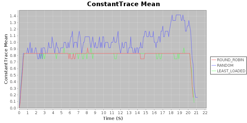
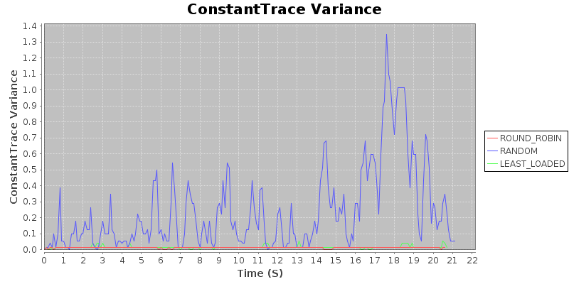
Trace 1: Constant Duration / Constant Arrival Rate
Result 1: Under uniform load, with sufficient compute to avoid backlog in an optimal assignment, random < round robin $\approx$ least loaded
This should not be particularly surprising. That a randomized approach should fail spectacularly is almost intuitive, as random assignment does a very poor job distributing load. Since the load is uniform (e.g. tasks take the same time to complete, and arrive uniformly), round robin and least loaded are more or less equivalent. This is born out in the following graphs, which show the average load and the variance of the load of the system over the course of a run, on a trace with a constant job duration and constant arrival rate. Takeaway: In situations where load is constant in duration and arrival rate, either of round-robin or least-loaded will work well.
This should not be particularly surprising. That a randomized approach should fail spectacularly is almost intuitive, as random assignment does a very poor job distributing load. Since the load is uniform (e.g. tasks take the same time to complete, and arrive uniformly), round robin and least loaded are more or less equivalent. This is born out in the following graphs, which show the average load and the variance of the load of the system over the course of a run, on a trace with a constant job duration and constant arrival rate. Takeaway: In situations where load is constant in duration and arrival rate, either of round-robin or least-loaded will work well.
|
|
Takeaway: In situations where load is constant in duration and arrival rate, either of round-robin or least-loaded will work well.
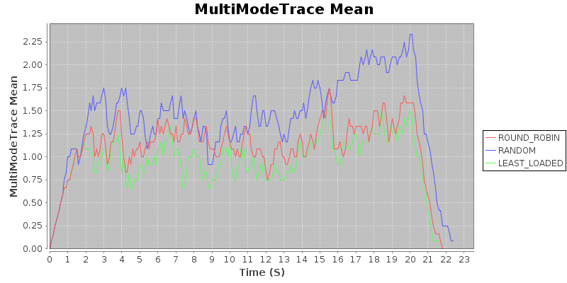
Trace 2: Modal Duration / Constant Arrival Rate
To analyze the load under slightly less stable conditions, I created a modal trace. Jobs take either 100, 500, or 1000ms, chosen uniformly at random for each job. Jobs arrive at a constant rate.
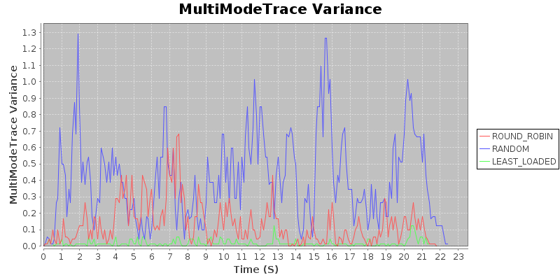
Result 2: With constant arrival rate and trimodal duration, random < round robin < least loaded.
Again, this should seem fairly intuitive. When the duration of jobs are not constant, round robin may assign more longer jobs to the same server, rather than packing them in optimally. We use a naive heuristic for least loaded (examining the number of outstanding jobs, rather than trying to estimate time to completion for jobs), and even so the least loaded algorithm achieves substantially better performance. In particular, note that the variance is very, very low, relative to the other two algorithms.
|
|
Takeaway: In situations where jobs arrive regularly, but duration is variable, use a least-loaded routing algorithm.
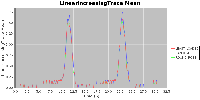
Trace 3: Constant Duration / Linearly Increasing Arrival Rate
To analyze the load under degenerate conditions, i.e. when the system becomes overloaded, I created a trace with constant job duration, and linearly decreasing interarrival rates, up to a maximum arrival rate threshold. The trace repeats twice.
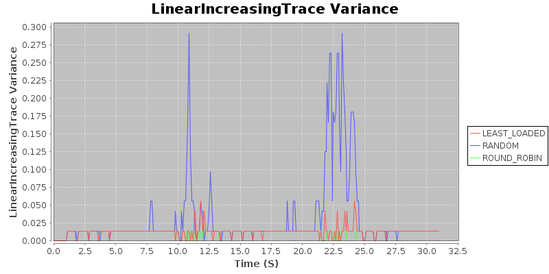
Result 3: Under degenerate conditions, random < round robin $\approx$ least loaded.
Note that all three algorithms produce very similar average loads. I find this to be quite surprising. The variance shows that random assignment does poorly, assigning jobs badly, while round robin and least loaded both keep variance very low. This suggests that if the trace were to have a higher cutoff for the interarrival rate, the mean would suffer for the randomized algorithm, but round robin and least loaded would stay more or less in lockstep.
|
|
Takeaway: If you are concerned about degenerate conditions when dealing with homogeneous jobs of about constant duration, use either the round-robin or the least-loaded routing algorithm.
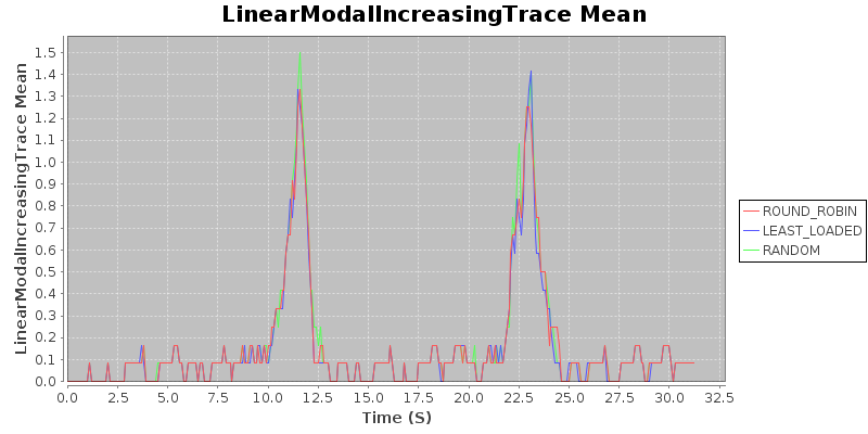
Trace 4: Modal Duration / Linearly Increasing Arrival Rate
Finally, to simulate somewhat more realistic degeneracy conditions, I combined the constant arrival modal trace with the linear increasing trace. The result is a trace with linearly decreasing interarrival rates (up to a threshold), with job duration sampled from $\{100, 500, 1000\}$ms, uniformly at random.
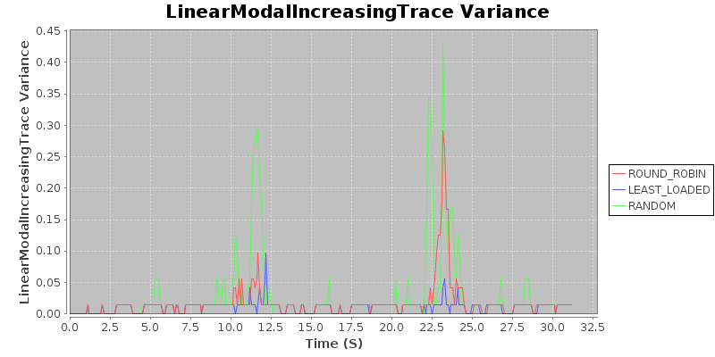
Result 4: Under realistic degenerate conditions, random < round robin < least loaded
Again, all three have similar means, but the variance tells. Here, we see that depending on the particular scenario, round robin may perform as well as least loaded (as in the first spike), which will occur when the optimal assignment happens to be the round robin assignment. But when the optimal assignment is different, round robin may perform quite poorly, as in the second spike, when the variance for round robin spikes. Our conclusion is that under heavy load, round robin would not degrade gracefully (and definitely not as gracefully as the least loaded balancer).
|
|
Takeaway: If you are concerned about degenerate conditions when dealing with heterogeneous jobs of varying duration, use the least-loaded routing algorithm.
Evaluating the Project
In my proposal, I said that I would build a framework, implement the centralized algorithms, and use the framework to do analysis answering questions comparing the different algorithms. In that proposal, I identified a fourth algorithm, in use at Indeed. After discussing with an expert in queueing theory (Professor Harchol-Balter), I determined that that their algorithm is not actually a load balancing algorithm (nor centralized), and is rather a time-sharing algorithm. Rather than comparing apples to oranges, I dropped the algorithm from the set of considered algorithms.
That said, I did achieve each thing I said I would do. I completed the framework, did the analysis, and was able to draw meaningful conclusions, providing numbers and data to back up naive intuition.
That said, I did achieve each thing I said I would do. I completed the framework, did the analysis, and was able to draw meaningful conclusions, providing numbers and data to back up naive intuition.
References
[1] O. Pearce, T. Gamblin, B. R. de Supinski, M. Schulz, and
N. M. Amato, “Quantifying the Effectiveness of Load Balance
Algorithms,” in International Conference on Supercomputing
(ICS’12), Venice, Italy, June 25-29 2012.

